FOCI vs Lasso on real-world dataset

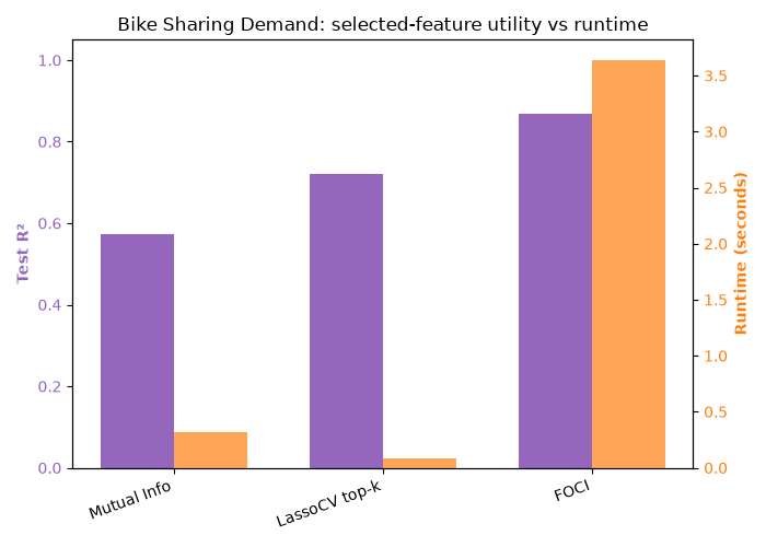
This example compares feature subsets selected by Feature Ordering by Conditional Independence (FOCI), Lasso, and a simple univariate mutual-information selector (as baseline) on a real-world regression task: hourly bike rental demand from the UCI/OpenML Bike Sharing Demand dataset.

Bike demand depends on calendar and weather variables and shows strong nonlinear and cyclical effects (e.g. time-of-day and weekday patterns), making it a useful sanity check for nonlinear feature selection.

We use a fixed chronological train/test split, a fixed five-feature budget for all methods, and the same nonlinear downstream regressor for evaluation. Lasso’s regularization strength is selected by cross-validation.

===========================================================================================
Feature selector comparison on Bike Sharing Demand (n=8690, p=12, k=5)
===========================================================================================
Method         | Time (s) | Test R²  | MAE      | Features
-------------------------------------------------------------------------------------------
Mutual Info    |    0.316 |   0.5745 |    95.19 | ['month', 'hour', 'temp', 'feel_temp', 'humidity']
LassoCV top-k  |    0.087 |   0.7212 |    79.76 | ['season', 'year', 'hour', 'temp', 'humidity']
FOCI           |    3.638 |   0.8673 |    51.71 | ['year', 'hour', 'workingday', 'weather', 'temp']
===========================================================================================

import time
from functools import partial

import matplotlib.pyplot as plt
import numpy as np
from sklearn.datasets import fetch_openml
from sklearn.ensemble import HistGradientBoostingRegressor
from sklearn.feature_selection import (
    SelectFromModel,
    SelectKBest,
    mutual_info_regression,
)
from sklearn.linear_model import LassoCV
from sklearn.metrics import mean_absolute_error, r2_score

from pyFOCI import FOCISelector

# -------------------------------------------------------------------------
# Config
# -------------------------------------------------------------------------
K_FEATURES = 5
STRIDE = 2  # for runtime reasons
TRAIN_FRACTION = 0.75
RANDOM_STATE = 0

# -------------------------------------------------------------------------
# 1. Load a real-world dataset
# -------------------------------------------------------------------------
bike = fetch_openml(
    "Bike_Sharing_Demand",
    version=2,
    as_frame=True,
    parser="pandas",
)
df = bike.frame.copy()

# FOCISelector and Lasso work on numeric arrays. The OpenML copy contains a few
# low-cardinality categorical columns, which we encode as deterministic integer
# codes. We intentionally do not add sinusoidal or one-hot feature engineering:
# the point is to compare feature selectors on a compact raw-feature view.
for col in df.select_dtypes(["category", "object"]).columns:
    df[col] = df[col].astype("category").cat.codes

# Runtime-only deterministic thinning. The original rows are hourly, so this
# keeps every second hour while preserving temporal order.
df = df.iloc[::STRIDE].reset_index(drop=True)

X_frame = df.drop(columns=["count"])
y = df["count"].to_numpy(dtype=float)
feature_names = X_frame.columns.to_numpy()
X = X_frame.to_numpy(dtype=float)

split = int(TRAIN_FRACTION * len(df))
X_train, X_test = X[:split], X[split:]
y_train, y_test = y[:split], y[split:]

# -------------------------------------------------------------------------
# 2. Feature selection benchmark
# -------------------------------------------------------------------------
selectors = [
    (
        "Mutual Info",
        SelectKBest(
            partial(mutual_info_regression, random_state=RANDOM_STATE),
            k=K_FEATURES,
        ),
    ),
    (
        "LassoCV top-k",
        SelectFromModel(
            LassoCV(cv=5, random_state=RANDOM_STATE, max_iter=20000, n_jobs=-1),
            threshold=-np.inf,
            max_features=K_FEATURES,
        ),
    ),
    (
        "FOCI",
        FOCISelector(
            max_features=K_FEATURES,
            min_delta=None,
            random_state=RANDOM_STATE,
        ),
    ),
]

results = []
w = 91
print("\n" + "=" * w)
print(
    "Feature selector comparison on Bike Sharing Demand "
    f"(n={len(df)}, p={X.shape[1]}, k={K_FEATURES})"
)
print("=" * w)
header = f"{'Method':<14} | {'Time (s)':<8} | {'Test R²':<8} | {'MAE':<8} | Features"
print(header)
print("-" * w)

for name, selector in selectors:
    t0 = time.time()
    selector.fit(X_train, y_train)
    elapsed = time.time() - t0

    support = selector.get_support()
    selected_idx = np.flatnonzero(support)
    selected_names = feature_names[selected_idx].tolist()

    # Same downstream model for all selectors: the comparison is about which
    # raw features are chosen, not about changing predictors between methods.
    predictor = HistGradientBoostingRegressor(
        max_iter=200,
        learning_rate=0.05,
        max_leaf_nodes=31,
        random_state=RANDOM_STATE,
    )
    predictor.fit(X_train[:, selected_idx], y_train)
    y_pred = predictor.predict(X_test[:, selected_idx])

    test_r2 = r2_score(y_test, y_pred)
    test_mae = mean_absolute_error(y_test, y_pred)

    results.append(
        {
            "name": name,
            "time": elapsed,
            "r2": test_r2,
            "mae": test_mae,
            "features": selected_names,
        }
    )

    print(
        f"{name:<14} | {elapsed:8.3f} | {test_r2:8.4f} | "
        f"{test_mae:8.2f} | {selected_names}"
    )

print("=" * w + "\n")

# -------------------------------------------------------------------------
# 3. Plotting results
# -------------------------------------------------------------------------
fig, ax = plt.subplots(1, 1, figsize=(7, 5))

names = [result["name"] for result in results]
r2_scores = [result["r2"] for result in results]
runtimes = [result["time"] for result in results]

x_pos = np.arange(len(names))
width = 0.35

ax_time = ax.twinx()
ax.bar(x_pos - width / 2, r2_scores, width, label="Test R²", color="tab:purple")
ax_time.bar(
    x_pos + width / 2,
    runtimes,
    width,
    label="Runtime (s)",
    color="tab:orange",
    alpha=0.7,
)

ax.set_title("Bike Sharing Demand: selected-feature utility vs runtime")
ax.set_xticks(x_pos)
ax.set_xticklabels(names, rotation=20, ha="right")
ax.set_ylabel("Test R²", color="tab:purple", fontweight="bold")
ax.tick_params(axis="y", labelcolor="tab:purple")
ax.set_ylim(0, 1.05)

ax_time.set_ylabel("Runtime (seconds)", color="tab:orange", fontweight="bold")
ax_time.tick_params(axis="y", labelcolor="tab:orange")

fig.tight_layout()
plt.show()