FOCI vs others on synthetic dataset

This example creates a small additive nonlinear synthetic dataset with redundant distractor features to demonstrate how Feature Ordering by Conditional Independence (FOCI) isolates complementary nonlinear signals, in comparison with some basic scikit-learn feature selectors.

Univariate feature selectors (SelectKBest) evaluate features marginally, ranking redundant collinear features equally high. Lasso is a (sparse) linear method, therefore does not work well on strongly nonlinear data, similar to Recursive Feature Elimination (RFE) with a linear model, which also cannot deal well with collinear features. Tree-based RFE works better, but is much slower and still dilutes split importances across collinear groups. A kernel-based method (SequentialFeatureSelector with Support Vector Regression) works well, but takes even longer.

================================================================================
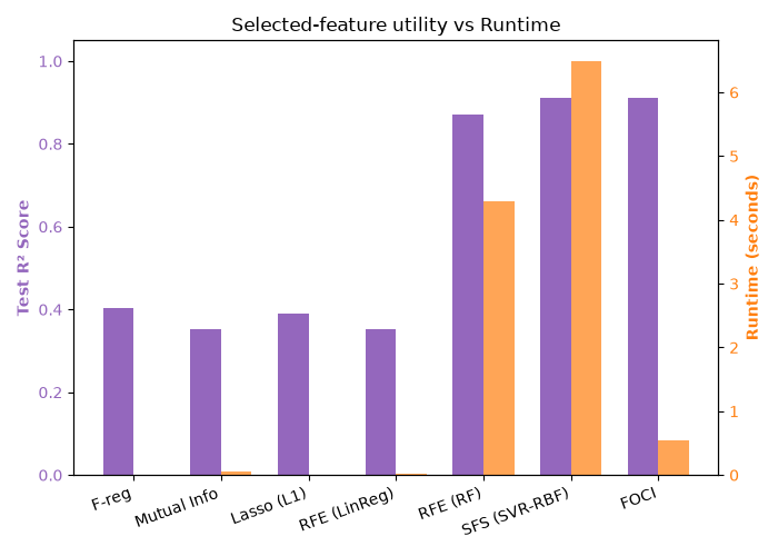
Feature Selector comparison on small additive nonlinear data (n=600, p=25, k=5)
================================================================================
Method        | Time (s) | Signal Cov | Test R²  | Sel Groups   | Sel Indices
--------------------------------------------------------------------------------
F-reg         |    0.001 |       0.50 |   0.4041 | x1,x2        | [1, 2, 10, 19, 24]
Mutual Info   |    0.056 |       0.25 |   0.3531 | x0           | [0, 4, 5, 6, 7]
Lasso (L1)    |    0.002 |       0.50 |   0.3897 | x1,x2        | [1, 2, 10, 19, 22]
RFE (LinReg)  |    0.015 |       0.25 |   0.3531 | x0           | [0, 4, 5, 6, 7]
RFE (RF)      |    4.283 |       0.75 |   0.8722 | x0,x1,x3     | [1, 3, 4, 5, 6]
SFS (SVR-RBF) |    6.489 |       1.00 |   0.9109 | x0,x1,x2,x3  | [1, 2, 3, 5, 7]
FOCI          |    0.545 |       1.00 |   0.9105 | x0,x1,x2,x3  | [0, 1, 2, 3]
================================================================================

import time

import matplotlib.pyplot as plt
import numpy as np
from sklearn.ensemble import RandomForestRegressor
from sklearn.feature_selection import (
    RFE,
    SelectFromModel,
    SelectKBest,
    SequentialFeatureSelector,
    f_regression,
    mutual_info_regression,
)
from sklearn.linear_model import Lasso, LinearRegression
from sklearn.metrics import r2_score
from sklearn.model_selection import train_test_split
from sklearn.pipeline import make_pipeline
from sklearn.preprocessing import StandardScaler
from sklearn.svm import SVR

from pyFOCI import FOCISelector

# -------------------------------------------------------------------------
# Config
# -------------------------------------------------------------------------
K_FEATURES = 5
N_DISTRACTORS = 4

# -------------------------------------------------------------------------
# 1. Generate small nonlinear dataset with collinearity
# -------------------------------------------------------------------------
random_state = np.random.RandomState(0)
n, p = 600, 25
X = random_state.normal(size=(n, p))

# Create a redundant collinear distractor group for x0
x0_distractors = range(4, 4 + N_DISTRACTORS)

X[:, x0_distractors] = X[:, 0:1] + 0.01 * random_state.normal(size=(n, N_DISTRACTORS))

# True underlying signals, all even.
y = (
    2 * (X[:, 0] ** 2 - 1)
    + 2 * (X[:, 1] ** 2 - 1)
    + 3 * np.exp(-X[:, 2] ** 2)
    + 2 * np.cos(2.0 * X[:, 3])
    + 0.1 * random_state.normal(size=n)
)

X_train, X_test, y_train, y_test = train_test_split(X, y, test_size=0.2, random_state=0)

# -------------------------------------------------------------------------
# 2. Benchmark comparison
# -------------------------------------------------------------------------
signal_groups = [
    {0, *x0_distractors},
    {1},
    {2},
    {3},
]
signal_group_names = ["x0", "x1", "x2", "x3"]

# Used for downstream evaluation and as the estimator for tree-based RFE
rf = RandomForestRegressor(n_estimators=100, random_state=0, n_jobs=-1)

svr_rbf = make_pipeline(StandardScaler(), SVR(kernel="rbf", C=10.0, gamma="scale"))

selectors = [
    ("F-reg", SelectKBest(f_regression, k=K_FEATURES)),
    ("Mutual Info", SelectKBest(mutual_info_regression, k=K_FEATURES)),
    (
        "Lasso (L1)",
        SelectFromModel(
            Lasso(alpha=0.01, random_state=0, max_iter=5000),
            max_features=K_FEATURES,
        ),
    ),
    (
        "RFE (LinReg)",
        RFE(estimator=LinearRegression(), n_features_to_select=K_FEATURES),
    ),
    ("RFE (RF)", RFE(estimator=rf, n_features_to_select=K_FEATURES)),
    (
        "SFS (SVR-RBF)",
        SequentialFeatureSelector(
            estimator=svr_rbf,
            n_features_to_select=K_FEATURES,
            direction="forward",
            n_jobs=-1,
        ),
    ),
    ("FOCI", FOCISelector(max_features=K_FEATURES, random_state=0)),
]

results = []
w = 80
print("\n" + "=" * w)
print(
    "Feature Selector comparison on small additive nonlinear data "
    f"(n={n}, p={p}, k={K_FEATURES})"
)
print("=" * w)
header = (
    f"{'Method':<13} | {'Time (s)':<8} | {'Signal Cov':<10} | "
    f"{'Test R²':<8} | {'Sel Groups':<12} | {'Sel Indices'}"
)
print(header)
print("-" * w)

for name, sel in selectors:
    t0 = time.time()
    sel.fit(X_train, y_train)
    dt = time.time() - t0

    support = sel.get_support()
    sorted_idx = [int(i) for i in np.where(support)[0]]

    selected_set = set(sorted_idx)
    selected_groups = [
        group_name
        for group_name, group in zip(signal_group_names, signal_groups)
        if (selected_set & group)
    ]
    selected_groups_str = ",".join(selected_groups) if selected_groups else "-"

    captured_groups = len(selected_groups)
    signal_coverage = captured_groups / len(signal_groups)

    if sorted_idx:
        rf.fit(X_train[:, sorted_idx], y_train)
        y_pred = rf.predict(X_test[:, sorted_idx])
        test_r2 = r2_score(y_test, y_pred)
    else:
        test_r2 = 0.0

    results.append(
        {
            "name": name,
            "time": dt,
            "r2": test_r2,
        }
    )

    print(
        f"{name:<13} | {dt:8.3f} | {signal_coverage:10.2f} | "
        f"{test_r2:8.4f} | {selected_groups_str:<12} | {sorted_idx}"
    )

print("=" * w + "\n")

# -------------------------------------------------------------------------
# 3. Plotting Results
# -------------------------------------------------------------------------
fig, ax = plt.subplots(1, 1, figsize=(7, 5))

names = [r["name"] for r in results]
r2_scores = [r["r2"] for r in results]
runtimes = [r["time"] for r in results]

x_pos = np.arange(len(names))
width = 0.35

ax_time = ax.twinx()
ax.bar(x_pos - width / 2, r2_scores, width, label="Test R² Score", color="tab:purple")
ax_time.bar(
    x_pos + width / 2,
    runtimes,
    width,
    label="Runtime (s)",
    color="tab:orange",
    alpha=0.7,
)

ax.set_title("Selected-feature utility vs Runtime")
ax.set_xticks(x_pos)
ax.set_xticklabels(names, rotation=20, ha="right")
ax.set_ylabel("Test R² Score", color="tab:purple", fontweight="bold")
ax.tick_params(axis="y", labelcolor="tab:purple")
ax.set_ylim(0, 1.05)

ax_time.set_ylabel("Runtime (seconds)", color="tab:orange", fontweight="bold")
ax_time.tick_params(axis="y", labelcolor="tab:orange")

fig.tight_layout()
plt.show()