Fuchs vs R-FOCI score normalization

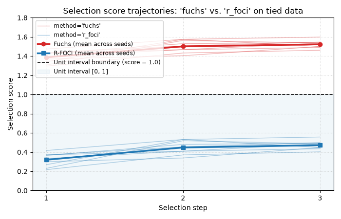
This example illustrates the difference in score normalization between the two scoring methods on discrete (tied) target data:

• method="fuchs" (the Fuchs 2024 closed-form score)

• method="r_foci" (matching the FOCI R reference implementation)

On tied target data, the continuous target rank-sum assumption in the Fuchs formula causes its score to be shifted upwards and frequently exceed 1.0. In contrast, the FOCI R reference implementation (method="r_foci") normalizes by the sample denominator \(S(y)\), keeping scores properly calibrated within the unit interval \([0, 1]\).

See Average vs. Max Ranking on Tied Targets in the User Guide for more information.

This example fits both methods across 10 seeds on a 3-level discrete target and plots the resulting score paths relative to the unit interval boundary.

Across 10 seeds on discrete target data:
  Fuchs  score range: [1.296, 1.598] (100.0% of step scores > 1.0)
  R-FOCI score range: [0.217, 0.557] (0.0% of step scores > 1.0)

import matplotlib.pyplot as plt
import numpy as np

from pyFOCI import FOCISelector

# -- config ----------------------------------------------------------------
N_SAMPLES = 350
N_FEATURES = 20
N_INFORMATIVE = 5
N_LEVELS = 3
NOISE_SIGMA = 0.5
K_FEAT_CAP = 3
N_SEEDS = 10


def make_data(seed, n=N_SAMPLES, p=N_FEATURES, n_levels=N_LEVELS, sigma=NOISE_SIGMA):
    rng = np.random.RandomState(seed)
    X = rng.normal(size=(n, p))
    y_lat = (
        2.0 * (X[:, 0] ** 2 - 1.0)
        + 1.5 * np.sin(2.0 * X[:, 1])
        + 2.0 * np.exp(-X[:, 2] ** 2)
        + 1.5 * X[:, 3] * X[:, 4]
        + 1.0 * (X[:, 3] >= 0)
    )
    y_lat += sigma * rng.normal(size=n)
    q = np.quantile(y_lat, np.linspace(0, 1, n_levels + 1))
    q[0] -= 1e-9
    q[-1] += 1e-9
    y = np.digitize(y_lat, q[1:-1]).astype(float)
    return X, y


# -- evaluate scores across seeds ------------------------------------------
fuchs_scores = []
rfoci_scores = []

for s in range(N_SEEDS):
    X, y = make_data(s)
    sel_f = FOCISelector(
        method="fuchs",
        rank_method="max",
        max_features=K_FEAT_CAP,
        min_delta=None,
        random_state=0,
    ).fit(X, y)
    sel_r = FOCISelector(
        method="r_foci",
        rank_method="max",
        max_features=K_FEAT_CAP,
        min_delta=None,
        random_state=0,
    ).fit(X, y)
    fuchs_scores.append(sel_f.score_path_)
    rfoci_scores.append(sel_r.score_path_)

fuchs_scores = np.array(fuchs_scores)
rfoci_scores = np.array(rfoci_scores)

# -- plot ------------------------------------------------------------------
fig, ax = plt.subplots(figsize=(7, 4.5))

steps = np.arange(1, K_FEAT_CAP + 1)

# Plot individual seed trajectories
for s in range(N_SEEDS):
    ax.plot(
        steps,
        fuchs_scores[s],
        color="tab:red",
        alpha=0.35,
        lw=1.0,
        label="method='fuchs'" if s == 0 else "",
    )
    ax.plot(
        steps,
        rfoci_scores[s],
        color="tab:blue",
        alpha=0.35,
        lw=1.0,
        label="method='r_foci'" if s == 0 else "",
    )

# Plot mean trajectories
ax.plot(
    steps,
    fuchs_scores.mean(axis=0),
    "o-",
    color="tab:red",
    lw=2.5,
    label="Fuchs (mean across seeds)",
)
ax.plot(
    steps,
    rfoci_scores.mean(axis=0),
    "s-",
    color="tab:blue",
    lw=2.5,
    label="R-FOCI (mean across seeds)",
)

# Reference unit interval boundary
ax.axhline(
    1.0,
    color="black",
    linestyle="--",
    lw=1.2,
    label="Unit interval boundary (score = 1.0)",
)
ax.axhspan(0.0, 1.0, color="tab:blue", alpha=0.06, label="Unit interval [0, 1]")

ax.set_xlabel("Selection step")
ax.set_ylabel("Selection score")
ax.set_title("Selection score trajectories: 'fuchs' vs. 'r_foci' on tied data")
ax.set_xticks(steps)
ax.set_ylim(0.0, 1.8)
ax.legend(loc="upper left", fontsize=8.5)
ax.grid(True, linestyle=":", alpha=0.5)

fig.tight_layout()
plt.show()

# -- numeric summary -------------------------------------------------------
print(f"Across {N_SEEDS} seeds on discrete target data:")
print(
    f"  Fuchs  score range: [{fuchs_scores.min():.3f}, {fuchs_scores.max():.3f}] "
    f"({np.mean(fuchs_scores > 1.0):.1%} of step scores > 1.0)"
)
print(
    f"  R-FOCI score range: [{rfoci_scores.min():.3f}, {rfoci_scores.max():.3f}] "
    f"({np.mean(rfoci_scores > 1.0):.1%} of step scores > 1.0)"
)